(This example can still be cleaned up. When completed, it should look as nice and clean as the one for PyAMG.)
The source code for a slightly more complex version of this example is in the PYSIT_DIR/examples/HorizontalReflector2D.py
directory. You can either type the commands into the IPython console,
or you can copy sections in by copying the text and using the %paste
IPython magic function.
ipython --pylab
First, we must import some fairly standard python and numerical python libraries that we will use in this demo. Run the following commands:
import numpy as np
import matplotlib.pyplot as plt
np), and the matplotlib plotting library which we
also abbreviate as is the standard.
Next, import all of the basic functionality of the pysit module:
from pysit import *
This will give access to almost everything we need. However, the gallery examples are not imported with the previous statement, so we must import thehorizontal_reflector module separately:
from pysit.gallery import horizontal_reflector
Pysit is designed to model the physical observation geometry in as accurately and as intuitively as possible. Generally the first thing that needs to be done is to define a physical, and computational, domain in which to work:
pmlx = PML(0.1, 100)
pmlz = PML(0.1, 100)
x_config = (0.1, 1.0, pmlx, pmlx)
z_config = (0.1, 0.8, pmlz, pmlz)
Currently, the PySIT supports Dirichlet boundaries and absorbing boundaries implemented using a perfectly matched layer, which
is defined using the PML class (as seem above). The PML is
specified in the same physical units as the domain. Here, we have
defined the PML to have length 1/10 units, in each direction, with a PML intensity
parameter of 100. Finally, we can define the domain itself:
d = RectangularDomain( x_config, z_config )
Pysit works for 1, 2, and 3D problems. We have chosen a 2D example. The argument list to the domain constructor is a configuration tuple for each dimension. The constructor uses the number of these configurations to determine the dimension of the problem.
After the physical domain is specified, we must specify a computational
domain or a mesh:
m = CartesianMesh(d, 90, 70)
The Cartesian mesh takes a domain as its first parameter, and then the number of grid points in each dimension as the remaining arguments.Finally, create the reflector:
C, C0 = horizontal_reflector(m)
Here, we have acoustic model parameters defined such that C^-2 = C0^-2 + M. Thus, C is the true wave speed, C0 is the initial non-oscillitory model, and M, which is not returned, is the perturbation of the model. The model problem can be plotted by:vis.plot(C, m)
Theplot command used is part of the visualization tools
provided by PySIT. The result should be a figure that looks like
this: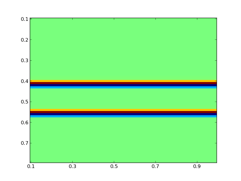 (Note that some gallery examples (Marmousi in
particular) generate the domain as well, but we must create one to use
the horizontal reflector gallery model.)
(Note that some gallery examples (Marmousi in
particular) generate the domain as well, but we must create one to use
the horizontal reflector gallery model.)
For this demo, we will use a single shot. A shot is a source coupled with a group of recievers. Before going on, let us extract some useful information:
zmin = d.z.lbound
zmax = d.z.rbound
zpos = zmin + (1./9.)*zmax
zmin and zmax are the rleft
and right (or top and bottom) physical boundaries of the
domain. Alternatively, we could hard code these from the specification
above, but this is a good time to introduce a useful property of the
domain. The spatial properties of the domain are typically described
without the boundary/ghost conditions. In this example,
d.z.lbound has the value 0.1 and
d.z.lbc.length has the value 0.1, so the
effective domain goes to 0.0 when boundary conditions are included (as
they are in wave propagation, exclusively).
shots = equispaced_acquisition(m,
RickerWavelet(10.0),
sources=1,
source_depth=zpos,
source_kwargs={},
receivers='max',
receiver_depth=zpos,
receiver_kwargs={})
shots is a list of Shot objects. Each
Shot object contains a source-reciever pair (or a Source-ReceiverSet
pair, to be more specific). Most of PySIT assumes that we are given
lists of shots, but perhaps this restriction should be lifted.
Pysit defines solvers as stateless objects that are handed to different
routines. This is so that all code that uses wave solvers remains
generic. Any pysit solver object can be used here, but we will use a
solver for the constant-density acoustic wave equation,
ConstantDensityAcousticWave. The constructor for
ConstantDensityAcousticWave automatically determines the
correct dimension for the solver based on the mesh m that
is provided.
solver = ConstantDensityAcousticWave(m,
formulation='scalar',
model_parameters={'C': C},
spatial_accuracy_order=2,
trange=(0.0,3.0),
use_cpp_acceleration=True)
wavefields = []
base_model = solver.ModelParameters(m,{'C': C})
generate_seismic_data(shots, solver, base_model, wavefields=wavefields)
vis.animate(wavefields, m, display_rate=10)
After the routine has run, each receiver (shot.receivers) will have its seismogram stored internally.To solve an inversion problem in PySIT, you must specify an objective function and an algorithm for optimizing it. PySIT currently defines the least squares objective in the time and frequency domains, as well as a hybrid approach. Objective functions require wave equation modeling, and thus are dependent upon our solver. Here, we define the time-domain objective:
objective = TemporalLeastSquares(solver)
PySIT defines inversion methods as stateful objects. Currently, PySIT supprts gradient descent, L-BFGS, and more, though L-BFGS is the preferred method:
invalg = LBFGS(objective)
initial_value = solver.ModelParameters(m,{'C': C0})
Next, we must configure the optimization routine's diagnostic recording. Each of the following dictionary entries specify the frequency with which the listed value is stored, as a function of iteration:
status_configuration = {'value_frequency' : 1,
'residual_frequency' : 1,
'residual_length_frequency' : 1,
'objective_frequency' : 1,
'step_frequency' : 1,
'step_length_frequency' : 1,
'gradient_frequency' : 1,
'gradient_length_frequency' : 1,
'run_time_frequency' : 1,
'alpha_frequency' : 1,
}
nsteps = 15
line_search = 'backtrack'
result = invalg(shots, initial_value, nsteps, line_search=line_search, status_configuration=status_configuration, verbose=True)
initial_guess using a backtracking line search. There are other optional arguments (that can be
seen in the documentation) that allow for extraction of intermediate values
and tracking of things like the residual history. Of course this will
need to run for hundreds (likely thousands) of steps to get a reasonable
result, but this gets the idea across.
Finally, we can plot the resulting model:
vis.plot(result.C, m)
Where you should see a figure that looks like this: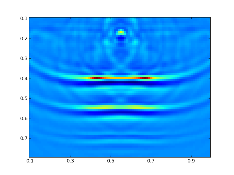
Additionally, you can look at the descent behavior of the algorithm by plotting the objective values:
obj_vals = np.array([v for k,v in invalg.objective_history.items()])
plt.figure()
plt.semilogy(obj_vals)
clim = C.min(),C.max()
plt.figure()
plt.subplot(3,1,1)
vis.plot(C0, m, clim=clim)
plt.title('Initial Model')
plt.subplot(3,1,2)
vis.plot(C, m, clim=clim)
plt.title('True Model')
plt.subplot(3,1,3)
vis.plot(result.C, m, clim=clim)
plt.title('Reconstruction')