Accurate and Efficient Computations with Structured
Matrices
Back
Description of the problem
Many practical problems, when modelled mathematically, are ultimately
reduced to a matrix problem--the solution to a linear system, an
eigenvalue or a singular value problem. The resulting matrix problem is
then solved in floating point arithmetic using
a conventional matrix algorithm such as the ones in
LAPACK or
MATLAB.
Limitations of the conventional matrix algorithms
These algorithms treat matrices as unstructured
and
deliver high absolute accuracy. This means that only
well conditioned problems are solved accurately. For example, only the
largest eigenvalues or singular values of a matrix are computed to high
relative accuracy; the tiny eigenvalues and singular values are
often lost to roundoff.
For example, computing the eigenvalues of the 100-by-100 Pascal matrix
using, e.g., eig(pascal(100)) in MATLAB yields the red curve in the
following figure

which is far from the correct answer---the blue curve (obtained by a call
to TNEigenValues(ones(100))).
The blue curve is symmetric, as expected, since the eigenvalues of the
Pascal matrix come in reciprocal pairs.
The need for accurate algorithms
No one can complain about getting the right answer, but this is
especially true when the desired quantity is very accurately determined by
the
data. In the example above, the smallest eigenvalue of the Pascal matrix is determined very accurately: it is the reciprocal of the largest one.
The smallest eigenvalues and singular values are often determined very accurately by the data, thus justifying the search for accurate algorithms for their computation.
How we design accurate algorithms
The first step is to find a structure-revealing
representation, i.e., a parameterization that reveals the matrix
structure (and hopefully determines the desired quantities
accurately).
For example:
- The bidiagonal Cholesky factor immediately reveals the
positive definite structure of a positive definite tridiagonal matrix and
determines its eigenvalues accurately;
Google the dissertation of Inderjit
Dhillon for more details.
- M-matrices are best represented by the offdiagonal elements and the
row sums. The row sums indicate the "diagonal dominance," a
crucial quantity in various applications. See my
paper with Demmel for details.
- Totally positive matrices are best represented as products of
nonnegative bidiagonals. See my paper for
details.
The second step is to arrange the computations in such a way that
subtractive cancellation does not occur. This is typically possible by
making some conventional matrix algorithms operate directly on the
parameters in the structure-revealing representation.
For example, to perform Gaussian elimination with complete pivoting on an
M-matrix, one computes separately, the offdiagonal elements and the row
sums of the Schur complement (which is also an M-matrix); see our
paper.
The need to avoid subtractive cancellation
Subtractive cancellation is the most common reason for loss of relative
accuracy. It occurs when two intermediate, nearly identical quantities
(known with certain uncertainty, say only to 10 digits) are subtracted.
The result may contain a lot fewer correct significant digits than the
summands; in fact, it may consist entirely of roundoff. It is interesting
that there is no rounding error generated by the subtraction in which subtractive cancellation occurs (see Demmel's 1997
book, problem 1.18 to see why). This subtraction is simply the messenger
revealing the loss of accuracy at earlier stages in the computation.
There is a lot of current research on the arithmetic expressions that can
be computed accurately in floating point arithmetic, but avoidance of subtractive cancellation has been a key
point in the development of the most recent high-relative accuracy
algorithms.
Matrix structures with which one can perform accurate
computations
- Totally nonnegative matrices
One can perform virtually ALL linear
algebra with totally nonnegative matrices to high relative accuracy. See
our paper as well as
preprint and
the MATLAB software.
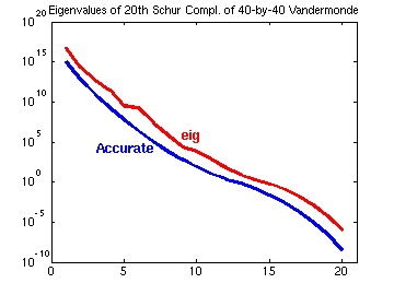
For example one can now compute the eigenvalues of the Schur complement of
a 40-by-40 totally positive Vandermonde matrix
(V(i,j)=(40-j+1)40-i+1) to high relative accuracy.
The conventional algorithms will not compute a single eigenvalue (not even
the largest one) with a single correct digit. See the next picture.
- Polynomial Vandermonde,
see our paper;
- Generalized Vandermonde,
see our paper;
- M-matrix,
see our paper;
- Semiseparable,
see our paper.