|
||
|
|
||
|
Suppose you want to fit a curve of degree j to k points with k - 1 > j. You may well fail to meet all the conditions, and find that no matter what polynomial of degree j you choose, you miss some ofĀthe points. You must then decide how you want to assess different kinds of errors; having done Āthis you may seek a "best" fit to the data within the class of polynomials you are examining.
In practice you may not know your data points with equal precision and may wish to scale errorsĀat different points differently you may wish to give certain points more weight in your computation than you give others. The approach we describe, in which all points are treated alike, is easily modified to handle whatever scales and weights you choose.
The least squares method we use has two nice features; first it is reasonable; second it is easy to do. We will derive simple expressions for the coefficients of the best polynomial.
Suppose you have n data points, (xj ,yj ), and you seek a best polynomial of degree k to fit the data. The answer depends on your criterion for being best.
A standardĀ procedure is to seek the polynomial of degree k that minimizes the sum of the squares of the errors. We can find the coefficients in this polynomial by the normal minimization technique of calculus: by setting the derivative of this sum with respect to each variable to zero.
These actions give us k + 1 linear equations for the k + 1 coefficients; their solution determines the polynomial.
This is what the equations look like:

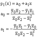
When k = 1, we can solve these equations and get the following solution:

Derivation of these expressions from the preceding equations is a straightforward exercise that you should perform yourself. In the k = 1 case, only the first two equations are needed.